Slow Burn Minsky Moments

Executive Summary

We seem to live in an era of rolling financial crisis. I suspect this is the result of a massive build-up of private sector debt. Sometimes these build-ups are accompanied by very high rates of credit growth, giving rise to a credit bubble. On other occasions, these build-ups sit simmering in the background, largely unnoticed until the proverbial s**t hits the fan, when they suddenly act as an amplifier causing a much steeper decline than would otherwise have been the case. I call these systemic vulnerabilities “slow burn Minsky moments.” Sadly, most markets appear to carry the fingerprints of these moments today. 

Of course, the timing of when they will matter (when the collective scales will fall from investors’ eyes) is completely unknowable. So, what is an investor to do? Some will choose to follow Chuck Prince’s ill-fated advice from prior to the GFC and keep dancing as long as the music is playing. For the more cautiously inclined, tail risk insurance is a more likely option. 

However, defining which risks you care about is, of course, vital. I’m assuming in this note that the risk is an equity market drawdown. In the past I’ve made the distinction between hedges (tightly correlated to the underlying event) and stores of value (strategies that pay off in the long term when the event occurs). The perfect insurance would exhibit both traits. 

One of the easiest tail risk hedges in this case is to hold cash. However, many seem to suffer FOMO and thus cash is often shunned, although with cash rates rising perhaps this will be less of an issue. The other large group of tail risk insurance is perhaps best described as negatively correlated with the event. The most obvious is a long volatility strategy. However, whilst this is an excellent hedge, it has been a truly terrible store of value (which in turn erodes its ability to be a hedge when we are faced with timing uncertainty). Effectively, running a long volatility strategy is the investment equivalent of death by a thousand cuts. 

Back in 2011 when I last wrote on this topic, I recommended a long quality/short junk position as a much more attractive vehicle for tail risk insurance. Such a position has a proven track record of being a good hedge (tightly negatively correlated with equity drawdowns) and back then had a tailwind in terms of valuation (making it a potentially good store of value). The hedge properties remain valid – quality has never failed to beat junk in an equity market drawdown. However, the broad quality factor is trading at the highest valuation extreme relative to its junk counterpart that we have witnessed since the early 1980s. This poses potential issues for its long-term store of value characteristic.

Value versus Growth generally does pretty well during equity drawdown events (especially if Financials are excluded). It isn’t as good a hedge as quality versus junk, but the valuation differential suggests it has good long-term store of value potential. To me this offers the best way of dealing with the timing uncertainty created by the prevalence of slow burn Minsky moments. 

The late, great Rudi Dornbusch once opined, “The crisis takes a much longer time in coming than you think, and then it happens much faster than you would have thought.” My own experience of premature bubble spotting certainly speaks to the first part of Dornbusch’s quote. And as we all know far too well, when looking through the lens of the short term there is no difference between being early and being wrong. 

This idea got me thinking about what I am calling “slow burn Minsky moments.” Recall that Minsky’s financial instability hypothesis holds that stability begets instability. In essence, I am referring to situations characterized by economically unsustainable processes or systemic vulnerabilities that build up during “good times” but carry within them either the seeds of their own destruction or create fragilities that exacerbate any external shock far beyond what may have been commonly expected. 

The fingerprints of slow burn Minsky moments

The typical fingerprint of a slow burn Minsky moment involves a build-up in private sector debt. This indicator also fits with the Minsky-Kindleberger bubble process that I have outlined many times over the years, where credit creation plays a major role in the development of a bubble (aka adding fuel to the fire). 

In his excellent The Next Economic Disaster, Richard Vague suggests that a ratio of private sector debt to GDP in excess of 150% is an important threshold. ¹  As Exhibit 1 shows, the U.S. has spent most of the last 20 years at or above this level! No wonder we have experienced a litany of financial crises over this period. 

EXHIBIT 1: U.S. PRIVATE SECTOR DEBT (% of GDP) 

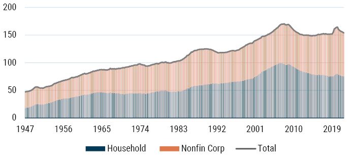
As of June 2023 | Source: BIS

Vague also points out that a period of rapid private sector credit growth is also a key concern (especially when combined with an already high private sector debt level). He suggests that a 5-year rate of growth in private sector credit to GDP of a level at or over 18% is a significant cause for concern (see Exhibit 2). 

EXHIBIT 2: 5-YEAR GROWTH IN U.S. PRIVATE SECTOR DEBT TO GDP 

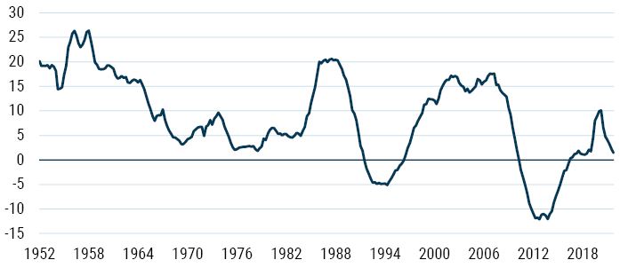
As of June 2023 | Source: BIS

The good news for the U.S. is that it isn’t anywhere near this level of growth. While this may help reduce the fear the U.S. is experiencing a “credit bubble,” personally I find the level of debt more worrisome from the perspective of slow burn Minsky moments. For instance, let’s imagine the U.S. enters a recession for some reason, something the lead indicators are telling us the U.S. is already experiencing (see Exhibit 3). In this scenario, the cash flows of the private sector are likely to fall significantly, easily turning a run-of-the-mill recession into something far more unpleasant. This is the nature of the systemic risk embedded in our economies today. 

EXHIBIT 3: CONFERENCE BOARD LEAD INDICATORS U.S. (YOY %) 

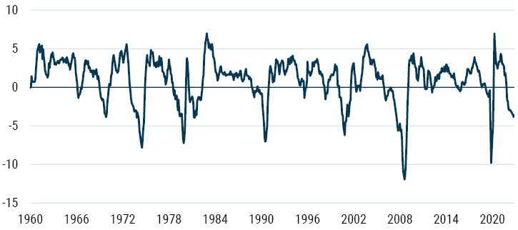
As of June 2023 | Source: DataStream

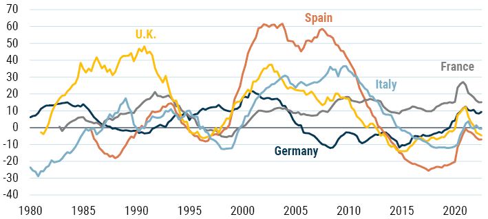
The U.S. is far from alone in facing this precarious predicament of dangerously high private sector debt to GDP. Exhibit 4 shows the private sector debt to GDP ratios for a variety of European countries. The U.K., Spain, and France all have levels of private sector debt to GDP greater than Vague’s warning threshold. Italy and Germany look to be in better shape than the others. 

EXHIBIT 4: PRIVATE SECTOR DEBT TO GDP RATIOS

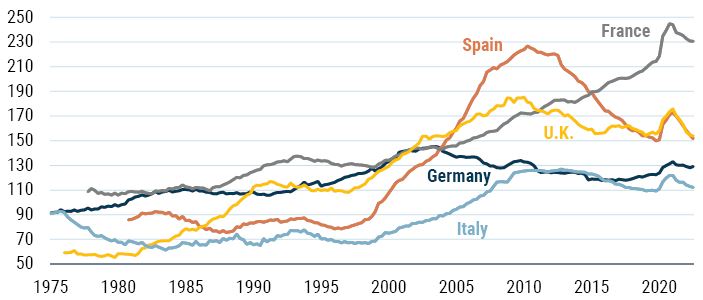
As of June 2023 | Source: BIS

As we saw with the U.S., the 5-year growth rate in the ratio of private sector debt to GDP is below the critical level identified by Vague in all the noted European countries in Exhibit 5. So, once again we have the fingerprints of a slow burn Minsky moment, but not of a massive credit boom. 

EXHIBIT 5: 5-YEAR GROWTH IN PRIVATE SECTOR DEBT TO GDP RATIOS 

As of June 2023 | Source: BIS

The last group I examined comprised Australia, Japan, and the Emerging Markets. Once again, we see a very similar picture: private sector debt to GDP ratios generally at or above the levels that Vague considers to be a warning sign of potential trouble ahead (see Exhibit 6). 

EXHIBIT 6: PRIVATE SECTOR DEBT TO GDP RATIOS 

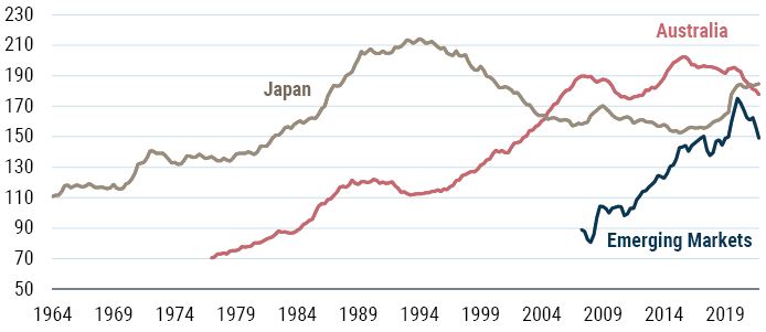
As of June 2023 | Source: BIS

When we look at the 5-year rate of growth in private sector debt presented in Exhibit 7 we see that Australia and the Emerging Markets look very similar to the trends we saw in the U.S. and Europe. However, perhaps surprisingly, Japan has the very dubious honor of hitting both of Vague’s warning levels, with a 5-year growth rate in private sector debt to GDP in excess of 18% as well as private sector debt to GDP ratio above 150% (actually at 185%). 

EXHIBIT 7: 5-YEAR GROWTH IN PRIVATE SECTOR DEBT TO GDP RATIOS

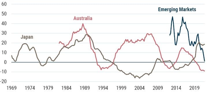
As of June 2023 | Source: BIS

Quick aside on Japan

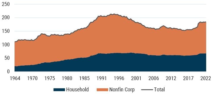
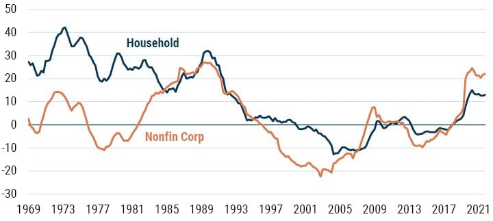
The Japan result surprised me. I wasn’t expecting to see Japan clear both the level and growth rate of private sector debt to GDP limits that Vague outlined. When I dug a little deeper, I found the following. In terms of the private sector debt to GDP ratio, it was both the corporate sector and the household sector that had been increasing debt. The increase was more marked in the corporate sector, with a 13-percentage-point increase since 2020, whereas the household sector had increased its debt by only 5 percentage points (see Exhibit 8).

EXHIBIT 8: JAPAN PRIVATE SECTOR DEBT TO GDP RATIO

As of June 2023 | Source: BIS 

In terms of the 5-year growth rate of debt accumulation (as a % of GDP), in Exhibit 9 we see the corporate debt to GDP growing in excess of 20% and household debt to GDP growing at around 13%. 

EXHIBIT 9: GROWTH OF JAPAN PRIVATE SECTOR DEBT TO GDP RATIO

As of June 2023 | Source: BIS

However, one major difference between the bubble experience that Japan lived through in the 1980s and the situation we see today concerns the overall position of the corporate sector. During the bubble years, Japanese companies were massive net borrowers. Today they are net savers. So, despite increasing its debt to GDP ratio, Japan is still actually saving more overall (see Exhibits 10 and 11). This may very well negate the superficial warning signs coming from the measures I have outlined here. I will address this further in a forthcoming paper about Japan. 

EXHIBIT 10: JAPAN SECTORAL BALANCES – CORPORATES ARE NET SAVERS 

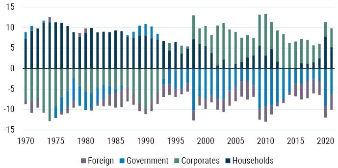
As of June 2023 | Source: MOF, GMO

EXHIBIT 11: JAPANESE CORPORATES – ASSET AND LIABILITY FLOWS (% OF GDP) 

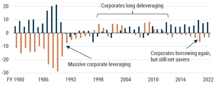
As of June 2023 | Source: MOF, GMO

Living in the shadow of a Minsky Moment

When we look around the world, we can see lots of countries that appear to be characterized by the problem of a slow burn Minsky moment: a chronic build-up of private sector debt that leaves the economic system extremely vulnerable. As I have opined countless times over the years, forecasting is a mug’s game. The future is, sadly, unknowable, so when these inherent vulnerabilities actually start to matter is beyond my ken. However, those who choose to ignore their existence are playing the same game as Chuck Prince, the ill-fated CEO of Citigroup, who, back in 2007 opined, “When the music stops…things will be complicated. But as long as the music is playing, you’ve got to get up and dance.” 

So, what do we do? As Pericles put it so well back in the 5th century BC, “The key is not to predict the future but to prepare for it.” I often talk about the need for robust portfolios (as opposed to optimal portfolios), which can survive a wide range of possible outcomes. Assuming we don’t want to follow the “just keep dancing” approach of Chuck Prince, how should we think about building portfolios when we know that systemic vulnerabilities exist? 

This question takes us to a world I last visited way back in 2011, ² the world of tail risk hedging. I stand by the approach I adopted in that paper. To wit, there are a number of questions we must answer when we consider tail risk protection. Essentially, they are: What? Why? How? 

What, why, and how (and when)

Let’s start with the verbal challenge my logic master at school would regularly hurl at me and my classmates as we struggled to make our case: “Define your terms!” What is the tail risk you are actually trying to protect yourself against? In general terms, the most common concern for investors is probably an equity market decline. However, for others it may be inflation. ³  Regardless, answering the “what” question is key before deciding the answers to the next two. 

The next question centers on asking “why” you are especially vulnerable to the particular risk you are trying to protect against. For example, why are you so sensitive to an equity drawdown? (Perhaps you are holding too many assets that effectively underwrite depression risk.) Or, why are you so worried about inflation? (What is your model for inflation and why are you so sensitive to its impacts?) 

The “how” question should be very obvious given you have defined the risk you care about as well as your rationale for caring about it. So now, how will you actually try to implement the protection you seek? Here we need to remember that tail risk protection is as much a value (or a contrarian) proposition as anything else in investing. That is to say that you should want to purchase tail risk insurance when it is cheap and no one else is interested in owning it. Most financial market behavior is best characterized by extrapolation, which effectively ignores the reality of a cycle. Thus, the average participants demand little payment for insurance during the good times because they can never see those times ending. Conversely, during bad times the very same participants are willing to overpay for insurance as they believe the bad times will never cease. 

For the purposes of this paper, I am going to stick with the concept of an equity market drawdown being the risk that scares most investors (the “what”). With reference to the “why” question posed above, it is worth noting Keynes’ insight: “Of all the maxims of orthodox finance, none, surely, is more anti-social than the fetish of liquidity, the doctrine that it is a positive virtue on the part of investment institutions to concentrate their resources upon the holding of ‘liquid’ securities. It forgets that there is no such thing as liquidity of investment for the community as a whole.” 

Thus chastened, we can consider the possible instruments one might use to mitigate the tail risk of equity market drawdowns. In my 2011 essay on this topic, I outlined three possible classes of tail risk protection that one might consider using. 

Cash. The oldest, easiest, and perhaps the most underrated form of tail risk hedge. Obviously, in a world where interest rates have been essentially zero (or worse), the cost of this particular form of insurance has been evident for all to see. As we move to higher rates, the opportunity cost of holding cash is reduced, and its appeal may rise once again. I will not separate out bonds from cash. A bond can always be unravelled into a string of cash rates, so unless you have a different view on the path of rates from the one implied, then the two assets are largely equivalent. 

Options/contingent claims. Occasionally, the market provides opportunities to protect against tail risk as a by-product of its manic phases. A prime example was the credit default swaps that were a result of the demand for collateralized debt obligations during the housing bubble of 2007. These instruments were priced on the assumption that there would never be a nationwide decline in house prices, and thus they provided a great opportunity for those who were concerned that such an outcome was more plausible than the market implied. Of course, such opportunities are far from guaranteed to exist; other classes of risk mitigation must also be sought.

Strategies with negative correlation to the tail risk event. For the specific type of tail risk (illiquidity/drawdown events) under consideration here, long volatility plays are often said to be negatively correlated. The simplest example of such a strategy is just to buy volatility contracts. However, as I have noted before, this strategy is the investment equivalent of death by a thousand cuts: you simply hemorrhage out over time as the roll return is usually negative. Just look at Exhibit 12, which shows that $100 invested in such a strategy in 2005 is worth just $0.004 dollars today! Most importantly, due to the erosion of capital over time, the ability of this kind of strategy to protect an investor obviously diminishes massively over time. This is an exceptionally expensive form of insurance. By its very nature, it is reasonable to assume insurance will have a negative expected value but, wow, this is pricey. 

EXHIBIT 12: RETURNS TO A LONG VOLATILITY STRATEGY

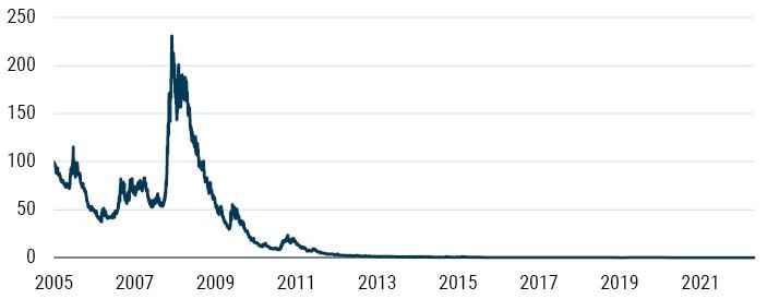
As of June 2023 | Source: Bloomberg

In my original paper of 2011, I presented a strategy that I thought had a much better chance of protecting investors. The argument I made was that a simple long quality/short junk portfolio had very similar insurance properties to a long volatility position but came with the added benefit of positive expected return (given the valuations at the time). I presented Exhibit 13 to highlight the nature of the close correlation in a given drawdown situation. 

EXHIBIT 13: LONG VOLATILITY VS. QUALITY MINUS JUNK

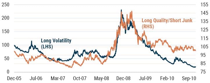
As of December 2010 | Source: Bloomberg, GMO

I have updated the exhibit to show how the strategies have evolved over the intervening years (see Exhibit 14). As we saw above, the long volatility strategy has proved to be an unmitigated disaster over the long term. However, the long quality/short junk factor portfolio has managed to deliver positive returns of around 4% p.a. over the same period.

EXHIBIT 14: LONG VOLATILITY VS. QUALITY MINUS JUNK

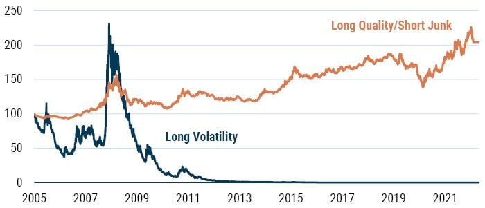
As of June 2023 | Source: Bloomberg, AQR

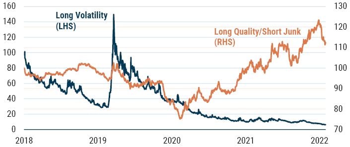
As Exhibit 15 shows, zooming in on the time period including the pandemic does little to alter the above picture. Yes, the long volatility strategy had a better payoff during the early stages of the pandemic, but quality relative to junk was also moving in the right direction, acting as a tail hedge once again. However, the differential performance during the pandemic recovery phase has been truly breathtaking. The rate of loss of the long volatility strategy is startling and couldn’t be more different than the performance of being long quality relative to junk.

In the parlance I have used previously, long volatility may be an excellent tail risk hedge but is undoubtedly an appalling store of value. In contrast, quality relative to junk looks to behave like both a tail risk hedge and a store of value (obviously depending upon the valuations). This ushers in the final question: the “when.” If you are going to deploy a long volatility strategy (like the one here) you need to ask the following: When will you put the protection in place and when will you remove it? 

Of course, if you knew the exact timing of a bad event, you wouldn’t really need tail risk protection as it would be your central case. However, as I have observed ad nauseum, those of us who follow a value-based approach don’t generally excel at what Ben Graham called the “way of timing.” Instead, we prefer to put our faith in the “way of pricing.” Or, as Howard Marks puts it, there are two schools of investing: the “I know” school and the “I don’t know” school (with value investors firmly in the second camp). These schools align with Graham’s “two ways” framework. This distinction is key if we are uncertain as to when an event might occur – exactly the conditions we face when dealing with slow burn Minsky moments.

If you know the future, great! Follow the way of timing. But for those of us with murkier crystal balls (or perhaps we are just more realistic about our ability to foresee the future), the way of pricing is inherently a much safer approach. Looking for strategies that offer insurance-like properties with a positive expected return is the way a value-orientated investor can approach the entire concept of tail risk protection. 

EXHIBIT 15: LONG VOLATILITY VS. QUALITY MINUS JUNK: THE RECENT PERFORMANCE

As of June 2023 | Source: MOF, GMO

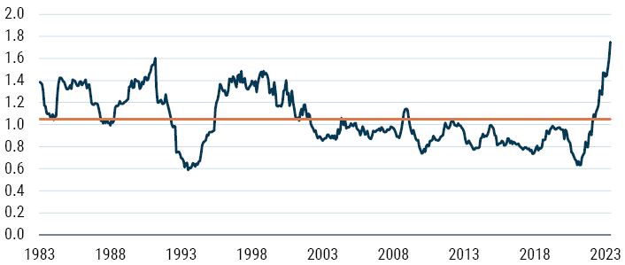
The only fly in the ointment for the quality factor relative to junk is its current valuation. Unlike when I originally wrote on the idea back in 2011 when the quality universe was priced at parity to junk, today simple quality is the most expensive relative to junk than it has been since the early 1980s.

Of course, a good correlation-based case for quality relative to junk can be made (i.e., it has always done well when needed). In the event of an equity market drawdown, will the quality factor outperform junk? History says this is more likely than not, but I worry it may not work as well as a long-term store of value as it has historically because of the current valuation (see Exhibit 16). ⁴

EXHIBIT 16: RELATIVE P/E OF U.S. QUALITY VS. JUNK

As of June 2023 | Source: GMO

This sends us off to see if we can’t find a possible alternative/additional store of value. Something that we at GMO have been (and remain) very keen on is Value relative to Growth. Indeed, as proof that great minds think alike (or perhaps fools seldom differ), Ben Inker has just written a paper on Value’s performance during recessions ⁵  that showed Value has had a pretty good relative performance during economic downturns (see Exhibit 17). 

EXHIBIT 17: RELATIVE PERFORMANCE OF VALUE (CHEAP HALF OF U.S. STOCK MARKET) IN RECESSIONS

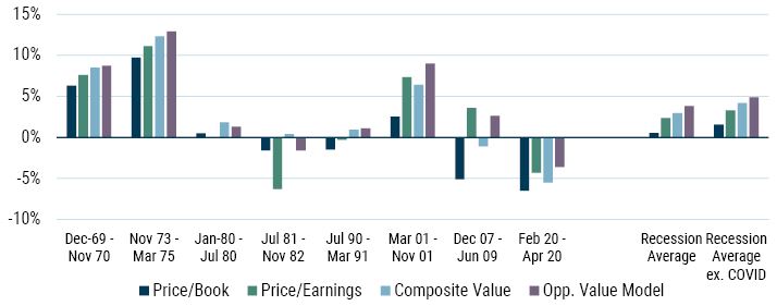
Data from 1969 – 2020 | Source: Compustat, Worldscope, NBER, GMO
Robust Value and Opp. Value Model are GMO proprietary value models.

My focus here is on general drawdowns in the equity market rather than recessions – although the two have some obvious overlap. Table 1 shows the performance of the U.S. equity market, U.S. Value minus Growth, U.S. quality minus junk, and cash over periods of notable equity drawdowns going back to the Great Depression.

As the table reveals, quality minus junk has been a very good tail risk protection strategy, generating positive returns during each drawdown listed. Value minus Growth does pretty well, with a couple of exceptions. I would generally characterize the periods of poor performance of Value relative to Growth during drawdowns as ones where the fundamentals of Value were open to question, even by stalwart value enthusiasts, and were, effectively, economic existential threats. For instance, during the Great Depression (1929-32) and in the aftermath of the housing bubble (2007-09), Financials turned out to be Value traps. They looked cheap on simple measures of Value, but that measure of Value was based on bubblelike economic times. ⁶

TABLE 1: PERFORMANCE DURING EQUITY MARKET DRAWDOWNS 

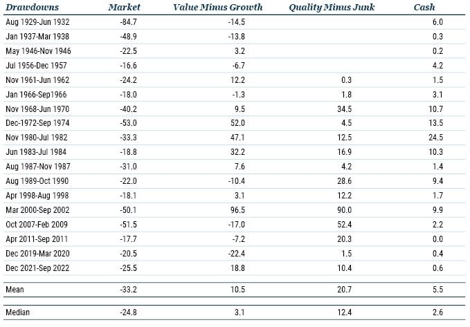
Source: GMO, Ken French, AQR

So, while Value relative to Growth isn’t as effective as the drawdown protection offered by quality relative to junk, I would argue that it has done a pretty good job and has had better returns during drawdowns than cash. Given the valuation appeal of Value versus Growth today (see Exhibit 18), there is a very clear case for using this as a protection against slow burn Minsky moments. Value today has a large margin of safety (especially deep value in the U.S. as Ben and team have explored recently in his June 2023 white paper and a webcast also in June). 

EXHIBIT 18: U.S. VALUE VS. GROWTH SPOT P/E 

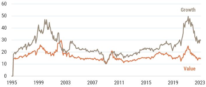
As of April 2023 | Source: Bloomberg, GMO

Of course, I have framed my discussion on tail risk protection from the perspective of an investor capable of exploiting long/short strategies. However, the general conclusions hold for those constrained to be long-only as well. I believe these investors, when faced with systemic vulnerabilities like slow burn Minsky moments, would do well to focus on assets with large margins of safety where the bad news has already been priced in as well as on the quality of the assets being bought. Today, this would suggest deep value and quality equities as good choices to consider within the U.S. market when thinking about trying to mitigate drawdown risk. My own preference – given my valuation bias – is obviously toward deep value rather than quality based on current valuations.

One final observation before I leave this topic. It concerns one more question: How much of your portfolio will you dedicate to tail risk protection? In my 2011 essay I asked how much of your portfolio you needed to dedicate to tail risk protection (using the long volatility strategy) in order to avoid the drawdown similar to the one associated with 2007-09. The answer, it turned out, was 30%. This seems to be a pretty reasonable rule of thumb. When I looked at the drawdowns that occurred subsequent to that original paper, 30% in tail risk protection seemed to do the trick in offsetting the respective equity declines. The notable exception was the drawdown between November 2021 and September 2022, which required a staggering 70% in tail risk protection to even get close to offsetting the drawdown! 

Conclusions 

This paper has sought to lay out a framework for spotting inherent economic vulnerabilities associated with the build-up of private sector debt. I term these slow burn Minsky moments. In the parlance of Bazerman and Watkins (2004), they are predictable surprises (aka Grey Swans). Such events have three defining characteristics: 1) at least some people are aware of the problem; 2) the problem gets worse over time; and 3) eventually the problem explodes into a crisis, much to the shock of most as they will say it’s a “Black Swan” event. In essence, the risk factor is clear, but the timing is uncertain. 

Timing uncertainty is nothing new to value investors. Sadly, we are all too accustomed to cheap assets getting cheaper, and more expensive assets getting more expensive. We follow what Ben Graham called “the way of pricing,” investing with a sufficient margin of safety to allow for errors in our timing and analysis (a natural form of risk protection), rather than the “the way of timing,” which involves guessing when things will happen. 

From the perspective of slow burn Minsky moments (and other predictable surprises), how should we seek to build robust portfolios? Simple long volatility strategies can be very effective hedges (i.e., their payoffs are highly correlated with the event risk), but they are truly lousy stores of value (their long-term performance is dreadful) as one might expect of an insurance policy. However, when we are faced with timing uncertainty (such as slow burn Minsky moments) they become largely unusable for this reason. 

I present three alternatives to long volatility strategies: cash (the oldest tail risk protection), a long quality/short junk strategy, and a long Value/short Growth strategy. All three can be priced relatively easily (i.e., we can construct valuation-based forecasts for their attractiveness) and all three generally pay off in the event of an equity market drawdown. To me, these seem to offer the best way to create robust portfolios. For the valuation-conscious investor, cash and deep value have the edge given today’s valuations.

Download article here.