This research is related to the newly launched Nebo platform, a portfolio construction tool that helps RIAs build better portfolios. Nebo bridges the gap between financial planning and asset management, and recently won the WealthManagement.com 2022 Industry Disruptor award.
Learn more about Nebo >
Executive Summary
Sequence of return risk is different from most other forms of risk borne by investors. It is not a risk inherent in an asset class, nor can it be seen in any portfolio analysis that looks at a single period of returns. As a result, it is not much of a surprise that sequence of return risk is entirely ignored in much of academic finance. But it is a meaningful risk for the vast majority of investment portfolios and there are useful tools that can mitigate its effects. We believe a portfolio construction framework that takes into account the lifespan of the portfolio and its expected cashflows can account for sequence of return risk better than any standard single-period optimization. And by dynamically reallocating portfolios in light of the returns assets have actually delivered and the consequent impact on their expected returns, portfolio managers can substantially further improve outcomes for their clients. Adopting these tools can be difficult, as both require combating natural human behavioral tendencies. But investors and their advisors would be well-served by at least understanding the ways those tendencies lead to sub-optimal long-term outcomes and determining whether it is worth some of the emotional pain involved in taking a different path.
As one of us points out relentlessly, risk isn’t a number, rather it is a notion or a concept. In the past, we have talked about the permanent impairment of capital as being the true risk you want to avoid. We have also highlighted the three paths that can lead to this outcome:
- Valuation risk. Buying an asset that is expensive means that you are reliant upon all the good news about that asset being delivered (and then some). There is no margin of safety in such investments.
- Fundamental risk. As Ben Graham put it. “Real investment risk is measured…by the danger of a loss of quality and earnings power through economic changes or deterioration in management.” We often talk of depression risk as a “deep” risk to equities because a depression can absolutely destroy the cash flows of stocks.
- Financing Risk. This is essentially anything that can force you to exit a position before you would otherwise choose to. For example, if you are using leverage, you can be forced to sell an asset because of, say, a margin call. One of the key features of financing risk is that it introduces path dependence.
In financial planning circles, one prominent “risk” discussion focuses on the sequence of returns. We will argue that sequence risk is actually a form of financing risk. The order in which returns occur will matter if (and only if) money is being added to, or withdrawn from, a portfolio. If no money is being added or withdrawn, there is no sequence risk. In this sense, sequence risk is not a risk inherent to a portfolio (as are valuation risk and fundamental risk) but depends on the external cash flows of the investor and is thus a financing risk. Hence the specifics of the risk – i.e., whether it’s better to have good returns followed by bad or bad returns followed by good – depends on whether you are withdrawing or contributing to your account.
But simply because sequence risk is a financing risk doesn’t make it any less real from an investor’s perspective. The evidence that financing risk/sequence risk matters is all too clear. Studies such as Morningstar’s “Mind the Gap” regularly show that investors achieve somewhere between 1 to 2 percentage points per year less in terms of return than their investment funds achieve – a gap generated by unfortunately-timed buy and sell decisions. Compound that over the kind of horizons involved in saving for retirement and it is little wonder that sequence risk is oft discussed by practitioners.
However, financing risk tends to get short shrift in academic finance circles. 1 It is generally assumed to not be an issue for anyone who is not investing with borrowed money. And indeed, for a “steady state” unlevered portfolio where money is neither being added nor withdrawn, there is no financing risk and no path dependence. But in the real world almost no portfolios fit that steady state model: as soon as money enters or exits a portfolio, financing risk and its consequent path dependence become an important issue.
Practitioners have long realized the salience of this path dependence. But understanding the existence of a problem does not imply success in mitigating it. Unfortunately, the tools of academic finance weren’t generally designed to handle this problem, leaving practitioners largely on their own to deal with sequence risk through heuristics and oversimplified simulations.
So, the question remains: how do we deal with it? This missive lays out two potential ways to mitigate sequence risk. The first is to start the investment process by asking the right question.
Framing Risk
When building a portfolio, it is important to clearly define the objective: what are you, the investor, trying to accomplish? In this sense, the portfolio is the answer. In standard finance theory, optimal portfolios are constructed to efficiently trade off return and volatility. This theoretical underpinning forms the basis for interactions with clients whereby questions are framed in terms of a client’s risk tolerance and/or risk capacity. This “risk tolerance” is then generally translated into a volatility limit (at odds of course, with the idea expressed above that risk isn’t a number). In this sense, the answer is driving the question, rather than the other way around.
As Inker and Tarlie (“Investing for Retirement: The Defined Contribution Challenge”) discuss, falling short of your financial needs is a much more intuitive framing of risk. In this framing, the right question is, “What do you need, and when do you need it?” It is not that volatility is inconsequential, as it is an important characteristic of the portfolio. However, volatility is not the primary driver of the portfolio. Instead, the primary driver is minimizing shortfall relative to suitably chosen targets that reflect the client’s wants, needs, and circumstances.
[Before moving on, it is worth pointing out that defining shortfall relative to suitably chosen targets does not mean that minimizing shortfall applies to problems only where the objective is to avoid falling below a basic level of subsistence. Because shortfall can be defined relative to any future set of targets spanning the investor’s horizon, the framework is useful, for example, for wealthy investors looking to compound their wealth for future bequests. Circumstances such as this are often framed in terms of risk capacity. But the concept of risk capacity is really just the other side of the “what you need/want” coin. One advantage of framing the problem in terms of needs or wants is that it is much more intuitive: asking someone what they need or want is a much easier conversation than asking them what their risk capacity is. Another advantage is that the needs/wants framing systematizes the portfolio construction process, directly aligning the financial plan with the portfolio in a way that the risk tolerance/risk capacity framing cannot.]
Framing risk as “not having what you need when you need it” and then constructing portfolios that minimize this risk does two things. First, the “what you need” question is the flip side of the risk capacity coin, framing the issue in terms of return rather than risk. Second, the “when you need it” question brings horizon into the problem. And bringing horizon into the problem can naturally address sequence risk. This is because when you frame risk in terms of shortfall, horizon enters the picture in two ways. The first is the total portfolio horizon, e.g., how long you expect to live. However, there is another horizon, and that is when you start caring about shortfall. And it is this second horizon that is the key to addressing shortfall risk.
If you have a long horizon until you care about shortfall, e.g., a 45-year-old saving for anticipated retirement at age 65 has 20 years until shortfall becomes a concern, sequence risk is not as big a deal as it is when your shortfall horizon is shorter. 2 As the 45-year-old ages and approaches retirement, concern about total portfolio horizon shrinks naturally. And as this horizon shrinks, a portfolio that minimizes shortfall reduces its weight in stocks in a way that still accounts for how much longer the 45-year-old expects to live.
This pattern is evident in the glidepath in Exhibit 1, which illustrates how the optimal shortfall portfolios change with age, assuming: 1) all assets are fairly priced; and 2) in the pre-retirement phase the asset owner desires to compound at 5% over inflation, and in the post-retirement phase at 3% over inflation. 3 In this chart we see that the weight in stocks falls at an accelerating rate as retirement age approaches, which, from the perspective of sequence risk, is an intuitive pattern. Framing risk as “not having what you need when you need it” and constructing portfolios that minimize this risk naturally accounts for the increased saliency of shortfall risk at retirement. In this way, framing risk as falling short of what you need and when you need it addresses, at least partially, sequence risk. 4
Exhibit 1: A “MINIMIAL SHORTFALL” GLIDEPATH
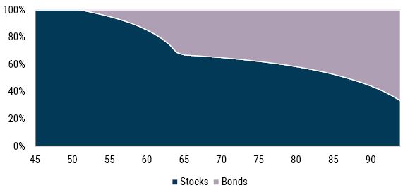
Source: GMO
Horizontal axis is age in years.
The second thing that can mitigate sequence risk is to “move your assets” based on how attractive they are. At its core, this behavior is nothing more than “buying low and selling high,” perhaps the most basic theorem of investing (and the key to protecting yourself against valuation risk). However, as Warren Buffett long ago observed, this is “simple but not easy.” Indeed, following this approach is anything but easy, as human nature has an uncanny habit of getting in the way (see Exhibit 2).
Exhibit 2: The psychology of “buy high/sell low”
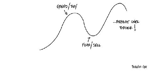
Source: Carl Richards – Behavior Gap
The tendency to follow the herd is a component of the human condition. There is strong evidence from neuroscience to suggest that physical pain and social pain are felt in exactly the same places in the brain. For example, in a study conducted by social psychologists Eisenberger and Lieberman, participants were asked to play a computer game. Players believed they were playing in a three-way game with two other players, throwing a ball back and forth. In fact, the two other players were computer controlled. After a period of three-way play, the two other “players” began to exclude the participant by throwing the ball back and forth between themselves. This social exclusion generated brain activity in the anterior cingulate cortex and the insula of the participants, both areas of the brain activated by real physical pain.
Contrarian strategies (like buying low and selling high) are the investment equivalent of seeking out social pain. In order to implement such a strategy, you will buy the assets that everyone else is selling and sell the assets that everyone else is buying. This is social pain. Eisenberger and Lieberman's results suggest that following such a strategy is akin to having your arm broken on a regular basis – not fun!
On the other side of the greed/buy fear/sell cycle, Bechara et al. provide us with some excellent evidence of the dark side of emotions. In this study, participants played an investment game. Each player was given $20 and had to make a decision each round of the game: invest $1 or not invest. If the decision was not to invest, the task advanced to the next round. If the decision was to invest, players would hand over $1 to the experimenter. The experimenter would then toss a coin in view of the player. If the outcome was heads, the player lost the dollar; if the coin landed tails up, $2.50 was added to the player's account. The task would then move to the next round with 20 rounds played overall.
This game was played with three different groups: “normals”; a group of players with damage to the neural circuitry associated with fear (target patients who can no longer feel fear); and a group of players with other lesions to the brain unassociated with the fear neural circuitry (patient controls). The experimenters found that the players with damage to the fear circuitry invested in 83.7% of rounds, the “normals” invested in 62.7% of rounds, and the patient controls 60.7% of rounds.
Was this result attributable to the brain's handling of loss and fear? Exhibit 3 shows the results broken down based on the result in the previous round as well as the proportions of the groups that invested. It clearly demonstrates that “normals” and patient controls were more likely to shrink away from risk-taking, both when they had lost in the previous round and when they had won! Players with damaged fear circuitry invested in 85.2% of rounds following losses on previous rounds, while normal players invested in only 46.9% of rounds following such losses.
EXHIBIT 3: PERCENT of players investing divided into the outcomes from the previous round
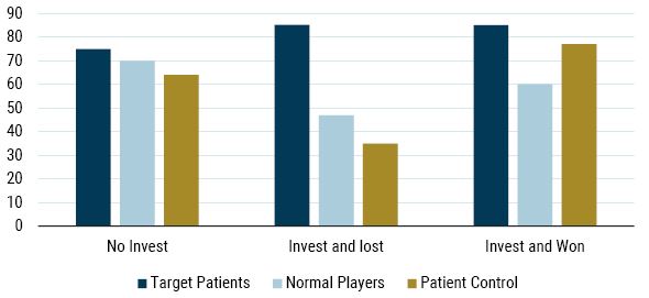
Source: Bechara et al. (2004)
So, while it may sound trite to invoke such an obvious aphorism as “buy low, sell high,” let alone elevate it to the level of theorem, it is actually incredibly hard to do. Yet, “buy low, sell high” is potentially a useful way to think about sequence risk.
The Basics of Sequence Risk
Viewing sequence risk as an example of financing risk helps us understand that sequence risk results from being forced to sell low or buy high, completely contrary behavior to the advice outlined above to buy low and sell high.
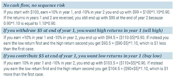
As we noted earlier, if there are no contributions or withdrawals from a portfolio, return sequence doesn’t matter. After all, a +10% return followed by a -10% return generates the same total gross return as a -10% return followed by a +10% return. 5
However, suppose you must pay bills at the end of year 1. In this case, it matters if you earn the +10% in the first year or the second year. An easy way to understand why this is true is to think of your bill payment as forcing you to sell some of your assets. Of course, as everyone knows, you want to sell high. But if you earn a low return in year 1, you are forced to sell low and you are worse off than if you earn a high return first and are able to sell high.
On the other hand, if you are in the accumulation phase and contributing to your portfolio, you are in the situation of forced buying. Given that you are better off buying low, you want the first-year return to be low and the second-year return to be high as you can see in the following scenarios.
The Derby
Perhaps the most salient sequence risk scenario occurs at retirement. In this case, the retiree has stopped working and is now dependent, at least in part, on withdrawals from their accumulated savings, which by this point are substantial. The added emotion of no longer generating labor income and being reliant on an accumulated nest egg adds to the saliency of sequence risk for people newly retired. More often than not it is this scenario that people have in mind when they think about sequence risk.
To study the sequence problem in more detail, let us set up a “Derby” in which we compare the performance of three different investment strategies. For each strategy, we start with a 65-year-old that has just retired with $1 million, in real terms. We then project 30 years into the future at various constant spending rates and ask whether the retiree runs out of money at any point over the 30-year period. 6 So, our measure of success for each running of the Derby is pretty simple: does the horse finish the race?
Because each Derby is run for 30 years, in order to get meaningful statistics, we need a reasonably long historical dataset. Robert Shiller's data for stocks and bonds, which extends back to 1881, allows us to run our Derby for all complete 30-year periods from 1881 to 2018. The probability of ruin is then the fraction of years in which the retiree's wealth falls below zero, i.e., the horse never finishes the race.
Table 1 summarizes the assumptions we use for stocks and bonds in our multiperiod optimizations and in our Monte Carlo simulations. One unusual item in this table is “expected return volatility.” This item is important because when dealing with long-horizon investing, the volatility profile of multiperiod returns is influenced by expected return volatility, as well as the relationship between forecast errors and volatility of expected returns. See “Investing for Retirement II: Modelling Your Assets” for more details on this topic.
Table 1: ASSET CLASS CHARACTERISTICS
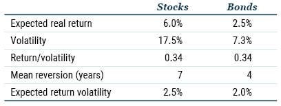
Source: GMO
The Three Horses
Exhibit 4 illustrates the three strategies. The first in the top left corner is representative of a commonly available glidepath that starts at around 50% weight in equities at age 65, declines to about 30% in the client's early 70s, and flattens out from there. Second, in the top right corner, is an optimal shortfall glidepath that starts with an equity weight around 60% that slowly declines as the client ages but that always assumes that assets are fairly priced. Third, in the second row, is an optimal shortfall approach that illustrates the stock and bond weights based on market conditions as they might evolve over the lifespan of the investor.
Exhibit 4: the three horses
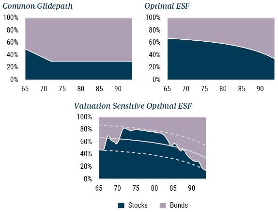
Source: GMO
Horizontal axis is age in years.
In principle, there is nothing inherently wrong with the Common Glidepath. The problem is not with the glidepath, per se, but with the fact that we don’t really know what problem the glidepath is solving. Said another way, to the extent that the glidepath is the answer, the issue is that we don’t know what the question is.
By contrast, the Optimal ESF glidepath is the answer to the question: what portfolio would I own as I age if my goal is to minimize shortfall risk, 7 assuming all assets are always fairly priced? And the Valuation Sensitive Optimal ESF strategy asks this same question but adjusts the portfolio weights every year based on minimizing shortfall risk, accounting for current market conditions, rather than assuming that all assets are fairly priced. This third graph is not a glidepath in the conventional sense as it illustrates the optimal shortfall stock and bond weights based on “real time” expected returns. To reflect the reality of career risk on the part of the portfolio manager or advisor, the stock weights are constrained to lie within ±20-percentage-point bands around the Optimal ESF weights, which serve as a benchmark of sorts. The solid gray line in this third graph illustrates the Optimal ESF stock weight, and the upper and lower dashed gray lines illustrate the upper and lower bounds. 8
Empirical Results
The top panel in Table 2 shows the results of running the Derby over all complete historical 30-year periods from 1881 to 2018. For withdrawal rates of 4% and 5%, the Common Glidepath horse fails to finish the Derby at a much higher rate than the other two horses. The Optimal Shortfall results show us that asking the right question – What do I need, and when do I need it? – and then minimizing the risk tied to the answer to this question leads to substantially improved outcomes.
Table 2: PROBABILITY OF RUIN
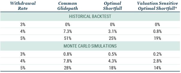
Source: Robert Shiller, GMO
*The stock weights in the Valuation Sensitive Optimal Shortfall results are constrained to lie between 20-percentage-point bands around the Optimal Shortfall stock weights (see Exhibit 4). For the historical backtests, the results for the unconstrained Valuation Sensitive Optimal Shortfall strategy are 0.7% and 18% for the 4% and 5% withdrawal rates, respectively. For the Monte Carlo simulations, the unconstrained results for the 4% and 5% withdrawal rates are 2.7% and 13%, respectively. Historical backtests use Robert Shiller data from 1926-2018. Monte Carlo results are based on 10,000 simulations.
By taking things a step further by moving your assets – i.e., owning more of the cheaper assets and fewer of the more expensive assets – we can do even better. This approach is very much tied to the framing of sequence risk in the previous section, where we viewed sequence risk as forced selling when prices are low or forced buying when prices are high. The obvious way to mitigate this risk is, to the extent possible, to sell the expensive assets if you are a forced seller and buy the cheap assets if you are a forced buyer. This is exactly the approach in the Valuation Sensitive Optimal ESF strategy.
One of the things we are always concerned about with historical backtests is the extent to which the results are driven by the relatively limited number of 30-year samples we have. To assess this concern, the bottom panel in the table shows the probability of ruin for Monte Carlo simulations designed to model a return-generating process that captures key elements of returns we have observed historically.
As detailed in “Investing for Retirement II: Modelling Your Assets,” modelling the return-generating process in a manner consistent with market history is not a minor point, especially when one is concerned about behavior over long horizons. Not only is it important to capture time-varying expected returns, it is also important to capture the shape of the volatility profile as the horizon changes. This last point is often overlooked but ignoring the fact that the volatility of bonds rises faster than the volatility of stocks leads to a distorted view that will tend to favor bonds over stocks at long horizons.
We see in the bottom panel of Table 2 that the Monte Carlo simulations replicate the basic pattern of the historical backtest that the probability of ruin for the Optimal Shortfall approach is about half that of the Common Glidepath, and the probability of ruin for the Valuation Sensitive Optimal Shortfall approach is about two-thirds that of the Optimal Shortfall approach. We also see in these results that history was particularly unkind to the 5% withdrawal strategy, an issue we will examine in greater detail below.
The probability of ruin results in Table 2 are an aggregate statistic over the entire horizon of 30 years, from retirement at age 65 until age 95. To unpack these aggregate results, the top two panels in Exhibit 5 show how “bad outcomes” (left panel) and “median outcomes” (right panel) for a 5% withdrawal rate vary with age. We see that for both bad and median outcomes, the age-specific results repeat the pattern of the aggregate probability of ruin results, viz. that the Valuation Sensitive Optimal Shortfall approach is superior to the Optimal Shortfall approach (which assumes all assets are always fairly priced), which in turn is superior to the Common Glidepath approach. In the left panel we see that while there is a small benefit at relatively short horizons of about 5 years (age 70) to holding fewer stocks in the event of bad outcomes, this benefit has disappeared by age 75. And as illustrated in the right panel, for median outcomes, holding fewer stocks when withdrawing at 5% is not better at any age. The bottom panels in Exhibit 5 shows how results vary with age for the Monte Carlo simulations. Comparing this exhibit with Table 2, we see that the Monte Carlo results exhibit the same pattern as the historical backtests, just as we saw for the probability of ruin.
Exhibit 5: OUTCOMES BY AGE
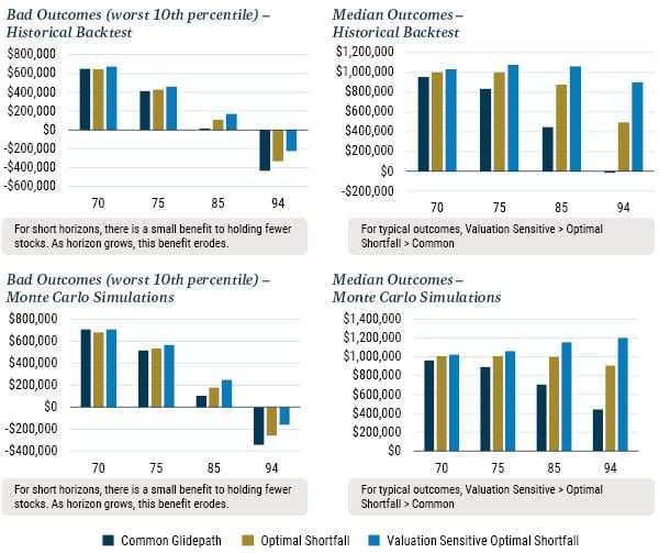
Source: Robert Shiller, GMO
Historical backtests using Robert Shiller data from 1926-2018. Monte Carlo results are based on 10,000 independent simulations. Starting asset base at age 65 is $1 million. Withdrawal is $4,167 per month ($50,000) regardless of asset base.
Two Periods in Detail
In this section we look at two time periods in detail. The first is dominated by the inflationary period of the 1970s when, in real returns, both stocks and bonds experienced a drawdown of approximately 40%. The second period is the Global Financial Crisis of 2008, wherein within a year the stock market fell by approximately 50%.
Retiring in 1970: the Problem Wasn’t Just Bad Hair and Bad Fashion
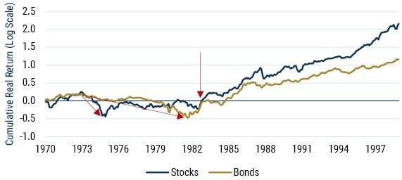
If one could choose a year to retire, it would not be 1970. As we can see in Exhibit 6, over the 1970s the cumulative real return on both stocks and bonds was negative. Stocks fell about 40% over a short period during the Nifty-Fifty crash of 1974, recovered somewhat, but still finished the decade under water. While bonds did not suffer a “crash,” they lost real purchasing power in a steady fashion as inflation relentlessly eroded value. This pitiful performance for both assets was the driver of the alarmingly high probabilities of ruin presented in Table 2.
EXHIBIT 6: STOCK AND BOND PERFORMANCE
Source: GMO
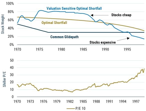
Returning to the Derby, the top panel of Exhibit 7 illustrates the stock weights for our three different horses. For the Common Glidepath and Optimal Shortfall portfolios, the weights depend only on horizon, and not on the state of the market. Not so for Valuation-Sensitive Optimal Shortfall, which after the Nifty-Fifty crash holds more equities than Optimal Shortfall, whose weight assumes equilibrium valuation. This excess weight persists for more than a decade, only falling below the equilibrium weight in the late 1980s. This pattern of weights for the Valuation Sensitive approach are consistent with equity valuation based on Shiller CAPE, which is illustrated in the bottom panel in Exhibit 7. Comparing the top and bottom panels we see that high equity weights are tied to low valuations, and vice versa.
For the Valuation Sensitive approach, the equity weights depend on the client’s needs and circumstances, and this manifests in a variety of different ways. 9 One is that portfolio weights depend on investment horizon – a way to think about this is that in the extreme case of a short horizon, e.g., one day, you would not want to own any stocks. But another aspect is the sensitivity of the portfolio weights to changes in expected returns. An intuitive and appealing feature of the multiperiod expected shortfall approach is that as investment horizon shrinks the weights become less sensitive to changes in expected returns.
EXHIBIT 7: STOCK WEIGHTS AND VALUATION
Source: Robert Shiller, GMO
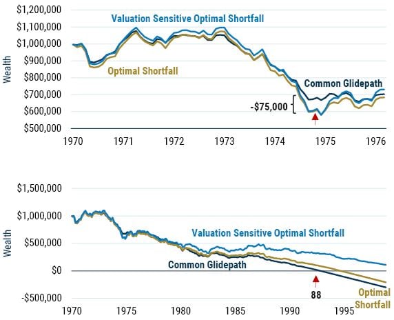
So, what impact do these weights have on portfolio value for a person starting with $1 million at age 65 and withdrawing $50,000 in real terms every year? As we can see in the top panel of Exhibit 8, the Common Glidepath’s lower stock weight does protect the portfolio in the first five years. The drawdown for the two shortfall approaches, which have similar equity weights over this period, is about $75,000 greater than that of the Common Glidepath. However, we can also see that this gap closes relatively quickly, within just a year or so.
In the bottom panel of Exhibit 8, we see how wealth evolves for these three strategies over the full sample. Starting around 1980, when the real returns for stocks and bonds start to diverge, we begin to see the divergence between the three strategies. The Common Glidepath starts to lag behind the other two strategies in the late 1970s, and this gap continues to widen as the high returns generated from owning cheap equities start to take hold. These equity positions generate returns that finance the required consumption of $50,000 each year, pushing out into the future the point of ruin. When the Common Glidepath runs out of money at age 88, the Optimal Shortfall strategy still has a balance in excess of $100,000, and the Valuation Sensitive Optimal Shortfall strategy has a balance in excess of $300,000.
EXHIBIT 8: EVOLUTION OF WEALTH
Source: GMO
The red arrow labeled “88” indicates that for the Common Glidepath, wealth turns negative at age 88.
Global Financial Crisis – Retiring into the Teeth of a Major Financial Crisis
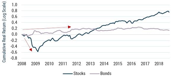
When thinking about the fear associated with sequence of return risk, one would be hard-pressed to come up with a more frightening scenario than the one that transpired during the Global Financial Crisis of 2008-09. As illustrated in Exhibit 9, someone retiring in 2008 was faced, right out of the gate, with a stock market that fell approximately 50% over a short period of time. Bonds, on the other hand, did just fine as they played their role as diversifier during the crisis, actually rising in value as stocks fell.
EXHIBIT 9: STOCK AND BOND PERFORMANCE
Source: GMO
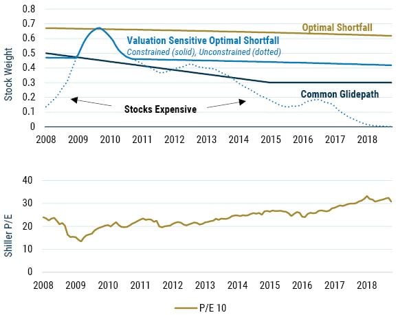
The top panel of Exhibit 10 illustrates the stock weights for our three different horses, along with the weight for the valuation-sensitive approach but with no constraint on the stock weight (dotted line). As before, for the Common Glidepath and Optimal Shortfall portfolios the weights depend only on horizon, and not on the state of the market. Not so for Valuation-Sensitive Optimal Shortfall, which had a low stock weight going into the crisis, not because of any particular view that there would be a crisis (although GMO was one of the firms sounding the alarm at the time 10 ), but because stock valuations were high, a Shiller P/E of around 25 according to the bottom panel in Exhibit 10. In the absence of constraints on the stock weight, valuation was high enough to warrant only an equity weight of around 13%, whereas the ±20% constraint band relative to Optimal Shortfall limited the stock weight to just under 50%, comparable to the Common Glidepath weight.
EXHIBIT 10: STOCK WEIGHTS AND VALUATION
Source: Robert Shiller, GMO
In Exhibit 11 we see the impact these weights have on portfolio value for a person starting with $1 million at age 65 and withdrawing $50,000 in real terms every year. As we can see, the Optimal Shortfall strategy fares worst, with a peak drawdown in 2009 of slightly more than 30%. The Common Glidepath’s lower stock weight does protect the portfolio, falling about $100,000 less. The drawdown in 2009 of the Valuation Sensitive Optimal Shortfall strategy is comparable to that of the Common Glidepath strategy, and because valuations revert to approximately 15x in 2009, the weight in this strategy briefly touches the weight in the Optimal Shortfall strategy. This means that this strategy’s wealth recovers quickly as stock valuations rise. The unconstrained Valuation Sensitive Optimal Shortfall strategy (dotted line) suffers a drawdown of only about 20%, owing to the low stock weight going into the crisis.
Following the crisis, the Optimal Shortfall strategy takes longer to recover, not because it has a lower weight in equity but because it has a substantially larger drawdown. Although the Common Glidepath suffers a lower drawdown than Optimal Shortfall, its lower equity weight in combination means that Optimal Shortfall catches up and overtakes in 2013. Continued strong equity returns propel the Optimal Shortfall strategy higher, eventually overtaking the Valuation Sensitive approach in 2017, whose weight in equities falls as the strong equity returns drive valuations higher.
EXHIBIT 11: EVOLUTION OF WEALTH
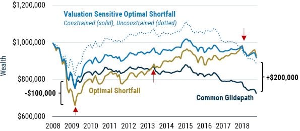
Source: Robert Shiller, GMO
By 2017, the optimal shortfall strategies are in a better position than the Common Glidepath as the lower equity weight of the Common Glidepath is simply not able to keep up with the high withdrawal of $50,000. For the unconstrained Valuation Sensitive strategy, the increased stock weight as equities recover leads to substantially higher wealth over much of the period. However, as stocks become more expensive, this strategy suffers from a lack of return, with wealth crossing below the Optimal Shortfall and constrained strategy in late 2017.
These results highlight one of the key points of this paper, which is that the investment strategy should be tied to the problem being solved. The answer, i.e., the portfolio, depends on the question! 11
Conclusion
If you are adding money to a portfolio, or withdrawing money from a portfolio, the order of the returns generated matters. We can think of this very simply using the basic theorem of investing which is “buy low, sell high.” If you are adding to a portfolio, you are a forced buyer so you prefer low returns early and high returns late. If you are withdrawing, you are a forced seller and you prefer the opposite.
In this paper we offer two suggestions, both of which we believe are basic principles. All portfolios, even those that lack cashflows in or out, stand to benefit from these suggestions. But portfolios with material cashflows, and for which sequence of return risk is particularly salient, stand to benefit the most.
First, you should be asking the right question. What is it that you want/need from your portfolio, and how do you minimize the risk that your portfolio does not deliver what you need when you need it? This requires rethinking risk. Typically, risk is thought of as volatility. But as we show in this paper, reframing risk as “not having what you need when you need it” can lead to substantially better outcomes simply because you are asking the right question. Furthermore, minimizing shortfall risk by incorporating two horizons – when you need the money and how long you need the money to last – goes a long way to naturally addressing shortfall risk when it matters most.
Second, you should be “moving your assets,” which is nothing more than an application of the basic theorem of investing (buy low, sell high). While this sounds trite, in reality it can be painful to attempt and most investors, professionals included, don’t even really try to. However, the outcomes can be so much better for the effort that we believe it is well worth the social pain inherent in always moving against the herd. Changing your allocations is also tied to the notion that if you are a forced seller, you should sell the expensive assets and if you are a forced buyer, you should buy the cheap assets. This will naturally tilt your portfolio in a more profitable direction and lead to better outcomes.
Download article here.
Register for full access to GMO's Research
The exception is papers discussing arbitrage and its limits, where portfolios are assumed to be levered and path dependent returns are a crucial factor.
In the 2015 GMO white paper “Who Ate Joe’s Retirement Money,” Chiappinelli and Thirukkonda show that the worst sequence outcomes are generally determined by what they refer to as the “Final 10 Years.” In the context of saving and investing for retirement, there are actually two “Final 10-Year” periods, one approaching retirement, and the other approaching longevity.
Framing risk as “What do you need, and when do you need it?” and constructing portfolios that minimize this risk defines what we call “Needs-Based Allocation.” See Investment Horizon and Portfolio Selection by Martin Tarlie :: SSRN for technical details.
The Nebo platform (www.nebo-gmo.com) is a fully open-architecture asset allocation platform that operationalizes the big idea that risk is “not having what you need when you need it,” and in so doing aligns a client’s plan with their portfolio in a way that allows advisors to construct personalized portfolios at scale.
This is because 1.10 * 0.90 = 0.90 * 1.10.
As an example, a 5% spending rate corresponds to spending $4,167 per month, in real terms. While this study is a bit unrealistic in that it assumes constant spending in real terms, it is an objective way to compare different strategies.
In this case, shortfall is defined relative to compounding at 3% over inflation.
In our studies we find that ±20-point bands are wide enough to capture the majority of the benefits of moving your assets.
The Nebo platform uses the multiperiod shortfall optimization framework to connect the financial plan to the portfolio to build a personalized portfolio for each client. It does so by combining market views with the needs and circumstances of each client, by defining concepts such as the Target Compounding Rate, i.e., at what rate does an asset owner need to compound wealth based on current wealth, target wealth, and anticipated cash flows. See www.nebo-gmo.com for more details.
See, for example, Jeremy Grantham’s 2Q 2007 Quarterly Letter “The Blackstone Peak and the Turning of the Worms: The Slow-Motion Train Wreck Continues,” available from your GMO representative.
See www.nebo-gmo.com for more details.