Executive Summary
The year 2019 was a very strong one for total returns in emerging debt. The EMBIG index of external debt was up 14.4%, amid falling credit spreads and sharply lower U.S. Treasury yields. The local debt GBI-EMGD index was up 13.5%, due mainly to strong returns in local rates, and broadly flat currency returns.
As a result of this performance, we now find stronger relative valuations in local currency debt. According to our valuation metrics, sovereign credit spreads have narrowed to the point where the added spread relative to expected losses from default is relatively thin compared with the historical experience. As for local debt, emerging currencies – which, despite the experience in 2019, are likely to be the key driver of returns for the asset class – look attractive based on our valuation metrics. In addition, despite the rally in local interest rates in 2019, interest rate differentials between emerging and developed markets remain consistent with recent historical norms. In other words, rates rallied nearly everywhere last year, so relative value did not change much.
In this piece, we update our valuation charts and commentary. We are happy to provide more detail on our methodology upon request.
External Debt Valuation
The rally in external sovereign debt in the fourth quarter caused valuations to deteriorate. As seen in Exhibit 1, the multiple of the benchmark’s credit spread to the spread that would be required to compensate for credit losses fell again over the course of the quarter. That multiple stood at 2.6x on December 31, 2019, down from 3.2x on September 30. Based on the historical experience of the past 25 years, this multiple of 2.6x is getting close to the level that we would deem unattractive. A ratio below 2.4x has, over the past 25 years, resulted in negative credit spread returns over the subsequent 24-month period 90% of the time.1 Over the course of 2019, the multiple declined from about 3.7x to 2.6x. As we’ve written in previous issues, this is due partly to compositional changes in the benchmark (e.g., addition of higher credit quality GCC countries) and a generalized spread compression.
Exhibit 1: Long-Term View of the “Fair Market Multiple” for Emerging External Debt
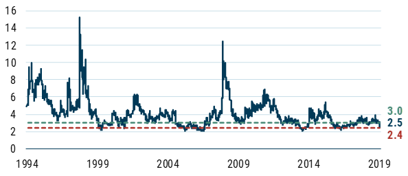
As of 12/31/19 | Source: GMO calculations based on Bloomberg and J.P. Morgan dataNote: Green line represents a credit multiple level above which EMBIG has subsequently delivered positive credit returns historically; red line represents a credit multiple below which EMBIG has subsequently delivered negative credit returns historically.
The main reason for the decrease in the multiple over the quarter was the ongoing decline in the EMBIG credit spread, which fell by 61 bps during the period, a very large move for just three months. This was due in part to a rally (lower spreads) in Argentina as the new government made positive announcements indicating a cooperative approach toward debt restructuring. It was also due partly to compositional changes, with Venezuela’s weight being reduced to zero. As for the change in the denominator of the multiple – the fair value spread – it was moderate over the quarter, increasing from 107 bps at end-September to 110 bps at end-December. Regular readers will recall that this fair value spread is a function of the weighted-average credit rating of the benchmark, along with data and assumptions on rating transition probabilities and recovery values given default. Over the course of the year, that fair value spread declined from 124 bps to 110 bps, based in part on the changes in benchmark composition that improved the credit quality of the benchmark. In terms of the fourth quarter, the fair value spread was influenced by a downgrade in Lebanon to CCC, and the above-mentioned rally in Argentina that was enough to meaningfully increase its weight in the benchmark. S&P’s placement of Brazil’s rating on positive outlook also influenced the fair market spread.
The preceding was a discussion of the level of spreads, or credit cushion. From a total return standpoint, the level and changes of the underlying risk-free rate also matters. In the fourth quarter, trends in U.S. Treasury yields were a negative contributor to benchmark returns, with the 10-year yield rising 24 bps. We measure the “cushion” in Treasuries by the slope of the forward curve of the 10-year swap rate, depicted by the light-font lines in Exhibit 2. The interest rate “cushion” (which we proxy as the slope of the forward curve) continues to be low by historical standards, meaning a sharp rise in the 10-year Treasury yield would be a surprise to the market. The slope of the 10-year forward curve ended the quarter at 18 bps, higher than the 8 bps of the prior quarter. We would view this as a slight positive relative to the previous quarter.
Exhibit 2: 10-Year U.S. Treasury Swap Curves at Quarterly Intervals
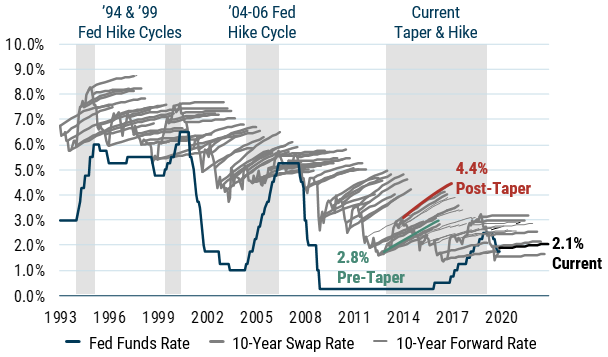
As of 12/31/19 | Source: GMO
Note: Projections as of each date, including those that are beyond 2015, are future prices as determined by the market and are not a GMO projection.
Local Debt Markets Valuation
Exhibit 3 provides a snapshot of our currency valuation methodology. The underlying model analyzes trends in macroeconomic fundamentals such as balance of payments composition and flows, valuation of the currency, and the economic cycle, via an econometric analysis, to come up with an estimate of total expected FX returns for each country in the GBI-EMGD benchmark. These are then combined into a single value of a total expected FX return using a weighted average of currencies in the GBI-EMGD. We then deduct the GBI-EMGD weighted carry from the estimated GBI-EMGD weighted value of total FX expected return to get to an expected EM FX spot return. Finally, we estimate a neutral range based on the backtest of the overall model to assess whether EM currencies are cheap, rich, or fairly valued. A value that is higher (lower) than the upper (lower) value of the neutral range could potentially indicate “cheap” (“rich”) currencies. A value that is within the neutral range would be considered “fair.” Based on our framework, EM currencies are attractively valued relative to the past five-year average.
Exhibit 3: GBI-EMGD Expected Spot FX Return Given the Fundamentals
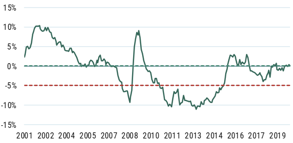
As of 12/31/19 | Source: GMO
Note: The values shown above apply the GBI-EMGD weights to the emerging currencies.
The expectations provided above are based upon the reasonable beliefs of the Emerging Country Debt team and are not a guarantee. Expectations speak only as of the date they are made, and GMO assumes no duty to and does not undertake to update such expectations. Expectations are subject to numerous assumptions, risks, and uncertainties, which change over time. Actual results may differ materially from those anticipated in the expectations above.
Exhibit 4 provides a snapshot of our traditional currency valuation methodology, which combines trends in the balance of payments and the real effective exchange rate, via a z-score analysis, and measures how far away current values are from their long-term averages. We keep our traditional valuation model in order to monitor the valuation of the USD and EUR. According to this methodology, the EUR and USD are currently in neutral territory in terms of valuations. Neither currency looks overvalued relative to their historical norms.
Exhibit 4: Value Score USD and EUR
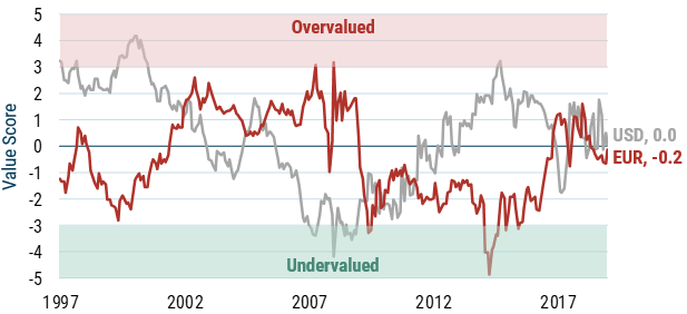
As of 12/31/19 | Source: GMO
Note: The value scores shown above apply the GBI-EMGD weights to the emerging currencies. GMO calculates a currency’s value score using a combination of the currency’s trend real price and the country’s trend current account balance.
As for emerging market local interest rates, we consider differentials in real yields to gauge the relative attractiveness of EM against developed markets (see Exhibit 5 below). In this regard, the story that has been in place for many quarters (years, actually) remains as we can still see a substantial positive gap between EM and developed market real yields. That gap was virtually unchanged during the fourth quarter as emerging real yields rose only slightly to 1.94% from 1.85%. The spread between EM and U.S. real yields was essentially unchanged during the quarter, at 191 bps. This spread has been fairly stable for several years running. The 5-year average of this spread is 207 bps. By our calculations, the real yield in the U.S. rose to 0.0% in December from negative levels in September, but Japanese and European real yields remain firmly in negative territory.
Exhibit 5: Inflation-Adjusted Bond Yields
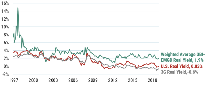
As of 12/31/19 | Source: GMO
Note: Real yields are measured using the country subindices of the GBI-EMD and GBI Global, respectively, less Consensus Forecast CPI.
Download to read the full article.